Conditional formatting is a feature in Cal – the spreadsheet component of Nebula Office, with which you can create all kinds of documents, drawings and spreadsheets.
Nebula Office is an all-in-one office productivity application. It is considered one of the best alternatives to Microsoft. With Cal, you can even edit spreadsheets and documents of Microsoft and Google. The user interface in Nebula Office is simple to use. Now let’s move on to conditional formatting on Calc.
What is conditional formatting?
To begin with, conditional formatting is a way of setting up cell formats. A sheet consists of various cells. A cell formed when a row and column intersect. When a format is changed based on a specified condition, it is conditional formatting.
This highlights the data which is outside your specification. Make sure you don’t overuse conditional formatting. This will reduce the impact of data which is outside that specification.
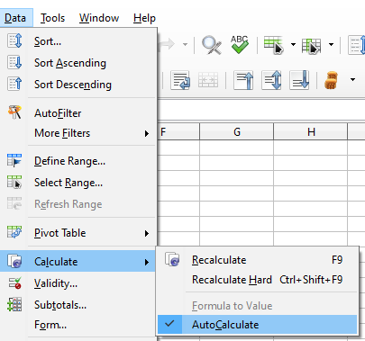
Remember to enable the AutoCalculate feature before starting the formatting. Now, let’s begin to know how to start conditional formatting.
Begin conditional formatting
- Enable AutoCorrect
- Go to Data>Calculate>AutoCalculate
- Now select those cells to which you need to apply conditional formatting.
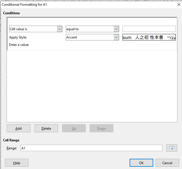
- Go to Format>Conditional>Condition.
- In the conditional formatting dialog box, click the Colour Scale.
- Now press data/data bar on the menu bar.
- Select Add and start creating a new condition.
- You can add as many conditions as required.
- In the Apply Style drop-down, select any style.
- The styles are already defined. You can repeat this as necessary.
- You can also use the New Style option to select styles.
- Press OK and close the dialog.
Now, conditional formatting will be applied to all the selected cells.
Management of conditional formatting
You can manage the cells that you have formatted. This is the management of conditional formatting.
- On the menu bar, go to Format>Conditional>Manage.
- This opens management of conditional formatting dialog box
- Here, select a range for the cells.
- Press Edit to save the changes.
- If you want to delete the conditional formatting, press Remove.
- To add a new definition to conditional formatting, select Add.
- Now click OK to apply all the changes.
Types of conditional formatting
There are four features to execute conditional formatting in Calc. These define the cells. You can select an option to declare a particular condition.
- Condition: This is the starting point for conditional formatting. You can define the format for data that is outside your specification.
- Colour Scale: This helps you set a background for your cells based on the value. This value is defined based on the data in the spreadsheet cell. The All Cells option is a must to use the colour scale. You can apply two or three colours for one conditional formatting.
- Data bars: You can use the Data bars to provide a graphical representation for a spreadsheet. This too is based on the values of data only. You can change the look of cells through More Options.
- Icon sets: An icon appears next to a data cell selected. This is for a visual representation to know the data range selected. Like all other types, you require the All Cells option. Different icons are available for you to select.
An example of conditional formatting
The main purpose of conditional formatting is to highlight certain cells. This helps in differentiating the data according to your need.
- Definition: To begin, you start with defining conditions. This is the same as the first step in beginning conditional formatting.
- Generating numerical values: As an example, create a table with various values. Make sure you use a formula =RAND() for a set of random numbers. Now, create a row of these numbers using that formula. Click on the cell and drag to define the range. Now you have obtained conditional formatting for this sheet.
- Define style: Apply style with the help of New Style option. Go to Format Cells and click Background. This applies background. You can define the style in the conditional formatting dialog box.
- Applying style: Once you have completed adding style and colour, apply it. Go to the conditional formatting dialog box and define your condition. For example, in the random numbers table, you can apply the style. If the value is less than 10 then format cell to Below. If the value is more than 10 then format cell to Above. This applies the specified condition to your sheet.