Formatting Data in Calc

Nebula Office is widely used software having multiple options to work with. It is a free office software for Windows and works fine with Google sheets, Google slides, and Microsoft office. Starting from sheets to documents to a presentation, you can get all of these features with the help of Nebula Office.

Any data organization is incomplete without Spreadsheets. An alternative to Microsoft Excel- Calc, a program under the Nebula office also helps us to work with Spreadsheets. It is much easier to work owing to the pre-designed templates and the advanced features.

This is a guide to Data Formatting using Calc.

Formatting Text

You can select the text and can adjust it within one cell by the following ways:

•       Select the cell or cell range.
•       Select Format Cells window or click Format > Cells from Menu or press Ctrl+1 to open the Format Cells Dialog box.
•       From the tabs mentioned, click Alignment.
•       Go to properties and select:

1. 1. 1. Wrap text automatically
      2. Shrink to fit cell size (to fit within cell borders)
      3. Manual line Breaks (use Ctrl+Enter while typing or Double-click and select the cell and move the cursor to the desired position of the line break).

•       Click OK.

Note:

Using a manual line break can cause overlapping of the text with the cell end as the width of the cell doesn’t change. To correct this, you have to manually adjust the cell width or reposition the text to prevent overlapping

 Formatting Numbers

You can do the number formatting in Nebula Office. The steps for the same are:

• Select Numbers Page under Format Cells window or select the cell.
• Click the icon to change the number format.
• Under the Category list, use any data type.
• Adjust the number of decimal places and leading zeros in Options.
• Enter the custom format code.

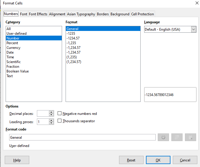
(You can do the local settings for different formats like data format and currency symbol from the Language setting menu.)

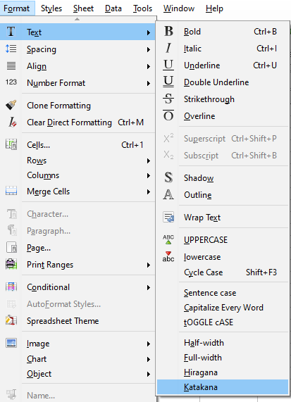
Changing Fonts, Style, and Size

Calc also provides the option of changing fonts and styles. The steps for it are as follow –

• Select the cell or cell range.
• Select the inverted triangle on the right side of the Font Name box and choose the font.
• Similarly, select the size from the Font Size box. The same can be done from the Format Cells menu also.
• Click B (Bold), I (Italics), or U (Underlined) for changing the font style.

Text Alignment

Alignment refers to the way the text is positioned to the cell edge. Choose any of the four options- Left, Center, Right, Justified.

Changing the direction of Text

Use the icons or Go to the Alignment tab under the Format Cells menu and select the Reference Edge option which changes the text as follows:

• Extension from the Lower Cell Margin – changes the text in the lowest cell edge externally.
• Extension from the Upper Cell Margin – changes the text in the highest cell edge externally.
• Text Extension Within Cells – changes the text in the cell.
• Select Vertically Stacked to make the text appear vertical.
• You can change the text direction from left to right and vice-versa using icons or by changing Text orientation to the desired angle with the indicator or by entering the degree in the Degrees box.

Adding Borders and Backgrounds to the cell

Adding Border to the text makes it more attractive. Background color helps in distinguishing the cells.

• Select the cell or cell range.
• Select Format Cells window or click Format > Cells from Menu or press Ctrl+1 to open the Format Cells Dialog box.
• Under the Borders tab, choose your desired border style and color.
• Under the Background tab, select the desired color from the palette.
• Click OK.

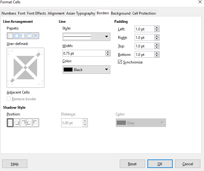
(You can also use icons under the Formatting Toolbar for similar changes.)

Formatting Cells and Sheet

Select the number of cells in rows or columns for formatting.

•       Click on Format > Cells.
•       Choose the desired format type and color from the menu.
•       Select the Formatting properties also.
•       Click OK.

Conditional Formatting

It helps to highlight a cell based on the data entered limiting to certain conditions.

•       Select the number of cells.
•       Go to Format > Conditional > Condition, Color Scale, or Data Bar.
•       Make the desired changes.
•       Click OK.

Note:

You can also Edit/Delete/Add the existing conditions by clicking Format > Conditional > Manage and making the changes.

An Overview

Data Formatting makes your sheet look ‘pretty’ and adds meaning. Channel your creativity with Calc, level up your skills, and master the art of making Spreadsheets.